The anatomy of efficient matrix multipliers

This post is the second of a three-part series about tract, Sonos’ open source neural network inference engine. In the first part, we explored the differences between training and inference paradigms, and how focusing on the inference problem can lead to some problem simplifications and solutions. This second chapter focuses on the most performance-critical part of a neural network inference engine: its matrix multiplication engine. We will discuss how neural networks translate to matrix products, then look at how matrix multiplication can be efficiently implemented on modern hardware.

Evaluating neural networks is a compute-intensive task. The graph of operators is just like a long list of mathematical expressions that have to be evaluated as fast as possible: once the network and input have been loaded into memory, it boils down to a lot of arithmetic operations and moving data around the memory.

From neurons to matrix multiplication

Knowledge of the underlying principles behind neural networks or just a bit of experimentation and profiling will lead to the same conclusion: all neural networks involve some form of matrix multiplications, and this operation is heavily weighted in the final breakdown of the computing cost.

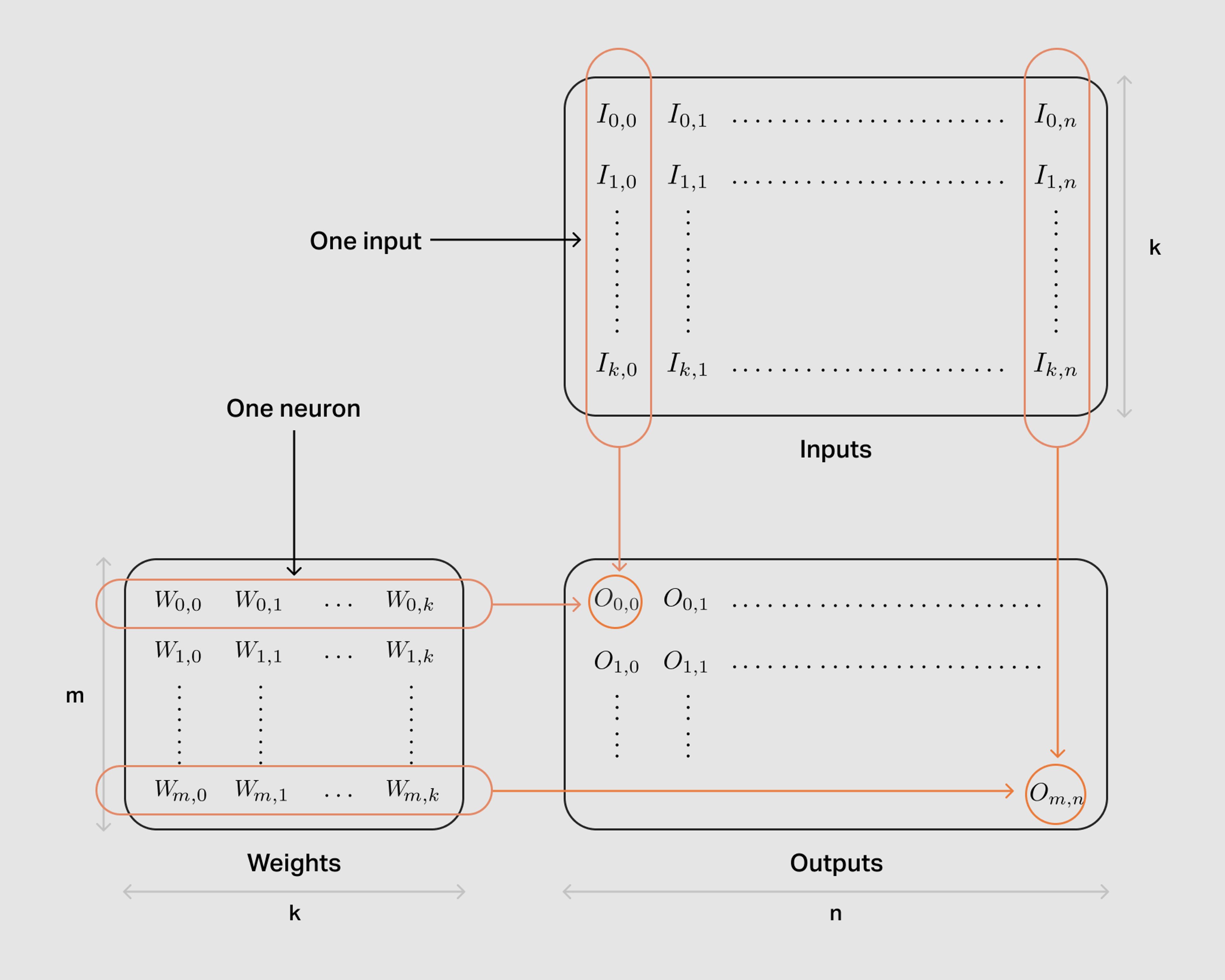
It’s not a big surprise: the “digital neuron” accepts a vector of numbers as input, multiplies each of them by a weight learned during training, before summing these products altogether.

Neural network layers typically contain dozens, or even hundreds of neurons, each using their own weights and operating on the same input and computing an output independently of the other neurons.

If we group the weight vectors of each neuron into a weight matrix, we get the textbook definition of a matrix-vector product.

Finally, if we apply the same neurons to more than one input at a time — a convolution does this for every pixel, for instance — then we get several input vectors that we can group together as a matrix. We are now running a matrix-matrix product: one operand is the trained weights for all the neurons, the other the input vectors all packed together. The output will also be a matrix: each column — for instance — will give the outputs produced by one given input, while each row will be emitted by a neuron.

As for the contents of the matrices, neural network theory operates on real numbers, with infinite precision. In the digital realm, floating point numbers are used as an approximation. Although 32-bit and 64-bit floating-point numbers operations are available on most modern chips, 32-bit is more than adequate for neural networks. While tract can also work with small 8-bit integers for quantized networks, this post focuses on the 32-bit floating-point case.

Matrix multiplication, software and hardware

The good news is that matrix multiplication is a very well-documented and understood class of problems, with countless research papers and libraries. Moreover, these problems are important enough and easy enough to describe that processor vendors design for them and advertise their performance. In the same way a car vendor uses the maximum speed or consumption to advertise their new model, processor designers or manufacturers work hard to demonstrate good performance on matrix multiplication. Multiplier circuitry occupies a large number of the transistors in a die, accounting for a significant portion of the chip cost. A lot of effort goes into ensuring software developers will be able to use them to provide the best experience to the end-user.

Specialized processors such as GPUs, TPUs and NPUs are designed to primarily deal with matrix multiplication. By targeting a specific domain, they can afford to make more hypotheses on the sub-structure of the problem. They may assume one of the two involved matrices is a constant may, or make hypotheses on the matrix sizes. This allows designing a highly efficient piece of circuitry to deal with the required sub-problem, but will be detrimental to the ability to re-purpose the device to another task that does not reside in the sweet spot.

CPUs, on the other hand, are intended to be general-purpose: their designers can not afford to pick their favourite sub-problem the same way. Instead, they provide generic building blocks that software developers or compilers must assemble to realize the required variation of matrix multiplication. A common building block on today’s CPUs is the “vector register”.

Vector Registers and SIMD

Registers are a key component of a processor: they act as its immediate memory. Data must be  moved from main memory to registers before the processor can perform arithmetic or logic operations on it, and the computed result will also be put in a register, before it can be stored back to memory.

CPUs have a handful of general-purpose registers that store just one number. These numbers can represent a memory address, a loop counter, a character, or many other things. The size of this number is 32 or 64 bits: the industry has been moving from 32-bit to 64-bit architectures over the past two decades. All laptops and desktops PCs are using 64-bit architecture today, most smartphones and high end recent embedded systems too, but 32-bit architecture are still there.

These general purpose registers are often complemented by vector registers: they are bigger in size, typically 128, 256, or 512 bits. As discussed earlier, we want to operate on 32-bit values: our vector register can hold 4 to 16 of these values. And critically, these registers come with instructions that can operate on all of the values or a vector at the same time. These instructions are often referred to as SIMD, for Same Instruction Multiple Data: they will operate on each “lane”, each of the four values, independently but doing the same thing.

Let’s consider the Arm v8 processor family: many high-end embedded systems and smartphones — and now even some laptops — are using these processors. They have 32 “general purpose registers”, and each can hold a 64-bit integer. The instruction set can manipulate them as memory addressing or integer quantities, but not for floating point operations.

These processors also feature 32 vector registers of 128 bits, with an instruction set designed to treat them each as vectors of four 32-bit floating point values. For instance, there is an “fadd” instruction that accepts two vector registers as inputs, interprets them as two vectors of 32bit floating point values, computes the four peer-to-peer addition in parallel, and stores the results as a new vector in a third register. Same goes for subtraction and multiplication. There are variants that operate on one vector input and one scalar input, using the same value repeatedly instead of working lane per lane.

Used correctly, this can yield a 4x speedup compared to performing operations on single values. This makes these SIMD instructions bigger building blocks than regular instructions that deal with just one value at a time. It is then up to the software developer (or their compiler) to put them together in the best way to realize the required operation.

Matrix multiplication and SIMD

A matrix multiplication operates on two matrices that share a common dimension. The output is a matrix whose dimensions are the two remaining dimensions from inputs. For instance, the product of an $m$-row, $k$-column matrix by a $k$-row, $n$-column matrix will yield a $m$ rows, $n$ columns matrix. Each value of the result will be the sum of the peer-to-peer products of values in the corresponding row in the first matrix with the ones from the corresponding column in the second. Computing one value in the output matrix requires $k$ scalar multiplications (and $k-1$ additions that do not really matter in the cost, as multiplications are much more expensive).

for col in 0..n {
    for row in 0..m {
        sum = 0;
        for i in 0..k {
            sum = sum + a[row * k + i]*b[i*n + col]
        }
        c[row * n + col] = sum
    }
}

As shown by the triple-level nested loop, the full matrix product requires $m*k*n$ individual multiplications. But the elementary multiplications are only the visible part of the iceberg. Matrix multiplication is also a memory-intensive operation: both input matrices are relatively big, and they do not fit on the limited storage offered by the CPU vector registers. The CPU has to read the matrix elements from main memory before doing the actual arithmetic. Reads are expensive in multiple ways. Firstly, because the memory is a linear space, the CPU can not load a value by its column and row pair. It needs to compute the actual offset in the buffer holding the matrix data row after row. Once this offset is known, the load instruction can be issued. Finally, reading from memory is slow: depending on how “lucky” we are, the data we load may be in the CPU cache, three to five cycles away, or deep in main memory, hundreds of cycles away.

This naive implementation, scanning the output matrix to compute its elements one per one, does $k$ reads from each of the two input matrices, repeating the process $m*n$ times. This would yield $2*k*m*n$ reads, each requiring a handful of instructions to compute the address, then issue the actual read, then wait for the load to happen, effectively drowning the $m*k*n$ multiplications in memory access.

The first trick: tiles

But there is a well-known trick. What if, instead of computing the output values one by one, we are computing them, say, on a tile of two-per-two?

for col in 0..n step 2 {
    for row in 0..m step 2 {
        sum00 = 0; sum01 = 0; sum10 = 0; sum11 = 0;
        for i in 0..k {
            a0 = a[row * k + i];
            a1 = a[(row + 1) * k + i];
            b0 = b[i*n + col];
            b1 = b[i*n + (col + 1)];
            sum00 = sum00 + a0*b0;
            sum01 = sum01 + a0*b1;
            sum10 = sum10 + a1*b0;
            sum11 = sum11 + a1*b1;
        }
        c[row * n + col] = sum00
        c[row * n + col+ 1] = sum01
        c[(row + 1) * n + col] = sum10
        c[(row + 1) * n + col + 1] = sum11
    }
}

We are now looping around the inner loop $n/2*m/2$ times instead of $n*m$. The inner loop still has $k$ steps, but each step now performs 4 products, so we still do $n/2*m/2*k*4=n*m*k$ multiplications. Just as expected.

The big difference is about the number of memory loads: the inner loop now has 4 of them, instead of 2 in the naive version, but it is run four times less often. We have divided the number of loads per two. It works because we can trust the compiler to be smart enough to put all the scalar variables in registers, so they can be used repeatedly without costing us more memory round trips.

Of course, we don’t have to stop there: we can make a bigger tile. The hard limit is the register size and number: we want all the “sum” variables for our tile to fit in CPU registers, and we also need to keep a few registers for the as and bs variables that store values from memory we will reuse. The 32 vector registers of an ArmV8 CPU can each hold four 32-bit values, giving us 128 slots to play with. A square tile of 8 values on each side uses half of the register space for the 64 accumulators, and requires twice 8 input values for as and bs. With this layout, the two outer loops will be $n$/8 and $m$/8 steps long, and the inner loop will perform 2*8=16 reads. We have moved from two reads per multiplication in the first approach to one read for four multiplications.

There is another benefit from this “tiling”. As we are now manipulating several values at the same time, we get opportunities to use the vector capabilities of our processor. First we have operations that will compute “fused” multiplication and accumulation over four lanes at a time: they read two vectors of four values each, compute the products lane-to-lane before adding in place these four values into another vector of value representing the “sums” variables.

The second trick: packing

Our optimization task is all about feeding the expensive multiplication circuitry as fast as we can.  By making a tile, we found a way to read less data from memory or read it over and over less often. Now we can focus on the inner tile body, and specifically the address computation: to read a value from A or B, we need to translate the column and row addressing to a buffer offset. This requires us to make relatively elaborate operations at each loop, which take cycles, and access data in complex fashion — specifically for A as the tile makes us read several rows in lock step.

We are not reading A or B just once: all values from A will be read as many times as the tile fits in the width of B. The big idea behind the packing is to rearrange the data from A and B before entering the loop, so that the values are in the order the tile will need them. Many CPU families have instructions that will read something from a given address and increment the address accordingly in one single step. Additionally, packing values from the inputs means we no longer need to load individual values, but can now load entire vectors.

As a result the favorable layout is a bit weird... We show the packing for the left A matrix. The red arrows represent the usual “row-major” order for a matrix storage: entire rows are stored left-to-right, consecutively from top to bottom. The black zig-zagging arrow represents the packed order: we group together little column vectors of length matching the height of the tile (4 here), moving left-to-right over a panel of 4 rows. Then we start again at the left for the next panel of 4 rows.

Despite requiring a preprocessing step, packing yields very good performance improvements… let’s try all of this.

Trying it out

We have written simple toy C multipliers to compare the performance of these tricks.

This graph shows the bandwidth of each of our multipliers, counting elementary multiplications only: the longer the bar, the faster the operation. Compared to the native implementation, the 4x4 packed implementation is roughly 8 times faster. However, there are a couple of unexpected observations:

• Firstly, the naive implementation outperforms the small tiles

• Additionally, the 8x8 packed implementation does not look good at all

What's going on here? The approach that we took is to write simple C code and compile it with optimizations. We rely on the compiler optimizer to figure out our operations can be translated to machine code using SIMD instructions everywhere. This compiler feature is called auto-vectorization, because it translates scalar source code to vector machine code. And it looks like it is doing a pretty good job making sense of the packed 4x4 implementation.

The packed 8x8 should be better than the 4x4. The Armv8 32 vector registers are enough to actually handle 12x8 tiles — that’s what tract production implementation uses. So what is happening here? In this case, the compiler optimizer has been outsmarted. It can not figure out how to arrange data in the vector registers to fully optimize our code so fallback to something that works but is not very efficient.

The progression following the unpacked tiling multiplier looks pretty nice -- except that the naive implementation beats the small tiles. Our guess is that, in this situation, the optimizer manages to actually do something smart with the naive implementation.

What we learn from this experiment is two-fold: first, tiling and packing works. Secondly, we can not blindly trust auto-vectorization. We will look into better alternatives in the third post of this series.

Off-the-shelf implementations

Not every project needs to go through all of this. There are easy to use, well integrated and efficient implementations of matrix multipliers available off-the-shelf: most of them will be found in BLAS-compatible libraries. BLAS is a pretty old thing, dating back from the Fortran years. It is a standardized API for linear algebra functions, one of them, called “sgemm”, is a 32-bit floating point matrix multiplier. It was ported to C and there are a few implementations of BLAS around, some open source like OpenBLAS, Atlas or BLIS, or shipped as part of operating systems  like in Apple Accelerate.

On this chart, we compare our toy naive and packed 4x4 implementations from before to BLIS, a relatively modern BLAS implementation. Off-the-shelf multipliers will be good enough for many use-cases, and for a little cost — will provide a nice speedup compared to a naive implementation.

What’s next ?

In this post, we have dived into the anatomy of efficient matrix multipliers, and seen how software and CPUs must work in synergy to realise efficient implementations for this ubiquitous problem. We have seen that relatively simple hand-crafted solutions can already be orders of magnitude faster than naive ones, but are still beyond the best available options.

In the final installment of this series, we will go deeper. We will look into versions of the tile code for Armv8.  We will show and discuss a bit of actual assembly code, and get acquainted with some specificities of two representatives of the Armv8 family: the venerable Cortex-A53 and the mighty Apple M1.